Accidents at Irongate
Now to review from the last post about the Chi Square Lesson. Question:
Data:

But why is the union concerned about whether one hour is more accident prone than another? A better question is to ask whether fatigue has an influence on accidents as the shift goes along. Thus we should see an increase in accidents as the hours pass by.
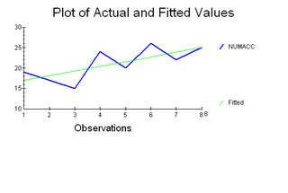
For the Microfit output for the Ordinary Least Squares Estimation (results), I used the following Equation:
NUMACC=B(1)+B(2)Shifthour+u(i)
And thus the Equation with the regression coefficients:
NUMACC=15.8571+1.1429Shifthour+u(i)
Like most regression equations the intercept coefficient has little relevance in this analysis. This would strictly mean that before work began during the zero hour that there would nearly 16 accidents. But the slope coefficient is predictive that for every hour the shift drags on that nearly 1.5 more accidents would occur.
And now to test how good this model is...
1. First let me test that the null hypothesis of the slope coefficient is equal to 0 (H0=0) and thus the alternative hypothesis is not equal to 0. If we test it at the 5% critical value (using the P statistics), then we reject the null hypothesis that the slope coefficient is equal to 0 which .05>[.047].
2. R^2=.50794 which signifies that over 50% of the variation in Numacc is attributed to which hour of the shift. And since there is only one slope coefficient then the same null hypothesis of that R^2 is not zero is the same at the .05 critical value [.047] of the slope coefficient.
And now to test whether our model passes the variety of diagnostic tests:
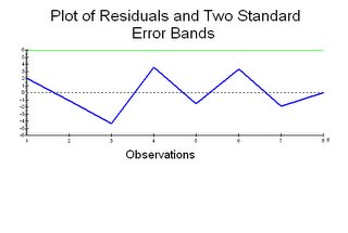
3. The Durbin Watson d statistic is stated as 3.0376. The dL=0.497 and dU=1.003 with n=8 and k=1. Since the d statistic is on the high side we need to figure the 4-dU=2.997 and 4-dL=3.503 and this means that it is in the zone of indecision as to whether there is evidence of negative correlation.
4. For the null hypothesis of no autocorrelation, we use the Diagnostic Test A and we do not reject the null hypothesis at the .05 level of significance (.05<.116 or .195). So even though the d statistic was indecisive this test resulted in no problem with autocorrelation.
5. For the Ramsey Reset Test/Diagnostic Test B, the null hypothesis is that the model is correctly specified which we do not reject at the 5% level of significance. Using the p statistics, we have .05<[.905] or [.928] by a wide range.
6. We now test for normality of the disturbance terms using diagnostic test C (Jarque-Bera test) with the null hypothesis that the population disturbance term is normally distributed. And here we sould not reject the null hypotheses at the 5% level of significance (.05<[.801]).
7. And lastly we test for heteroscedasticity with diagnostic test D. The null hypothesis of homoscedasticity cannot be rejected on the basis of the test at the .05 level of significance (.05<[.470] or [.541]).
So in conclusion we have an indecisive test for the Durbin-Watson d test for negative autocorrelation. But we can conclude at the 5% level of significance for any problems with first order autocorrelation (AR(1)) and autocorrelation and non normal population disturbances and lastly heteroscedasticity.
But it still would have been better to get all the raw data to do a complete analysis of the Accidents at Irongate.
And that is the way it is done.
The Irongate Foundry, Ltd., has kept records of on-the-job accidents for many years. Accidents are reported according to which hour of an 8-hour shift they happen. The following table shows their accident report.
Data:
The union at the foundry wants to know whether accidents are more likely to take place during one hour of the shift rather than another. They are asking you what you think.
Do you think that more accidents are likely to take place during one hour of a shift over another?
But why is the union concerned about whether one hour is more accident prone than another? A better question is to ask whether fatigue has an influence on accidents as the shift goes along. Thus we should see an increase in accidents as the hours pass by.
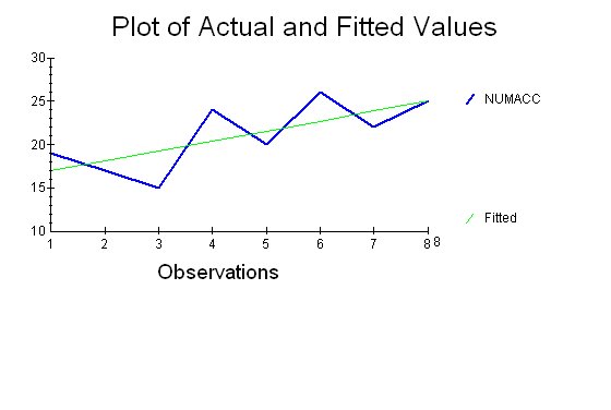
For the Microfit output for the Ordinary Least Squares Estimation (results), I used the following Equation:
NUMACC=B(1)+B(2)Shifthour+u(i)
And thus the Equation with the regression coefficients:
NUMACC=15.8571+1.1429Shifthour+u(i)
Like most regression equations the intercept coefficient has little relevance in this analysis. This would strictly mean that before work began during the zero hour that there would nearly 16 accidents. But the slope coefficient is predictive that for every hour the shift drags on that nearly 1.5 more accidents would occur.
And now to test how good this model is...
1. First let me test that the null hypothesis of the slope coefficient is equal to 0 (H0=0) and thus the alternative hypothesis is not equal to 0. If we test it at the 5% critical value (using the P statistics), then we reject the null hypothesis that the slope coefficient is equal to 0 which .05>[.047].
2. R^2=.50794 which signifies that over 50% of the variation in Numacc is attributed to which hour of the shift. And since there is only one slope coefficient then the same null hypothesis of that R^2 is not zero is the same at the .05 critical value [.047] of the slope coefficient.
And now to test whether our model passes the variety of diagnostic tests:
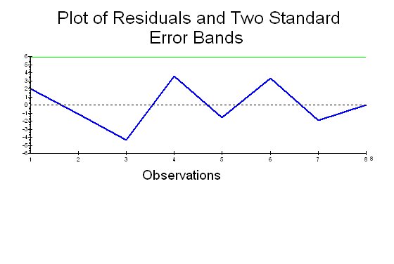
3. The Durbin Watson d statistic is stated as 3.0376. The dL=0.497 and dU=1.003 with n=8 and k=1. Since the d statistic is on the high side we need to figure the 4-dU=2.997 and 4-dL=3.503 and this means that it is in the zone of indecision as to whether there is evidence of negative correlation.
4. For the null hypothesis of no autocorrelation, we use the Diagnostic Test A and we do not reject the null hypothesis at the .05 level of significance (.05<.116 or .195). So even though the d statistic was indecisive this test resulted in no problem with autocorrelation.
5. For the Ramsey Reset Test/Diagnostic Test B, the null hypothesis is that the model is correctly specified which we do not reject at the 5% level of significance. Using the p statistics, we have .05<[.905] or [.928] by a wide range.
6. We now test for normality of the disturbance terms using diagnostic test C (Jarque-Bera test) with the null hypothesis that the population disturbance term is normally distributed. And here we sould not reject the null hypotheses at the 5% level of significance (.05<[.801]).
7. And lastly we test for heteroscedasticity with diagnostic test D. The null hypothesis of homoscedasticity cannot be rejected on the basis of the test at the .05 level of significance (.05<[.470] or [.541]).
So in conclusion we have an indecisive test for the Durbin-Watson d test for negative autocorrelation. But we can conclude at the 5% level of significance for any problems with first order autocorrelation (AR(1)) and autocorrelation and non normal population disturbances and lastly heteroscedasticity.
But it still would have been better to get all the raw data to do a complete analysis of the Accidents at Irongate.
And that is the way it is done.
posted by Ronald Rutherford at 2:16 PM
![]()
![]()


0 Comments:
Post a Comment
<< Home