Mundell-Fleming|Model Part One|IS-LM-BP Model

The LM schedule is an upward-sloping curve representing the role of finance and money. The initials LM stand for "Liquidity preference/Money supply equilibrium" but is easier to understand as the equilibrium of the demand to hold money as an asset and the supply of money by banks and the central bank. The interest rate is determined along this line for each level of real GDP.

Construction of the LM (Money Market Equilibrium) curve...
M(Supply Fixed)=M(Demand)=c(0) + c(1)Y - c(2)r
Which means that for equilibrium MS=MD which equals an autonomous amount c(0) and the transaction demand of money as a percentage of Income and "the opportunity cost of holding [cash] balances" which inversely affects MD by the interest rate r (this is often referred to as the speculative demand for money).
Factors that Shift the LM Schedule

Two factors that will shift the LM curve are changes in the exogenously fixed money stock and shifts in the money demand function.

1.

A shift in the money demand function means a change in the amount of money demanded for given levels of interest rate and income, what Keynes called a shift in liquidity preference.
...
A shift in the money demand function that increases the demand for money at a given level of both the interest rate and income shift the LM schedule (upward and) to the left.

2.

...an increase in the money stock will shift the LM schedule (downward and) to the right.

The LM Schedule: Summary
The LM curve:

1. is the schedule giving all the combinations of values of income and the interest rate that produce equilibrium in the MONEY MARKET.
2. Slopes upward to the right.
3. Will be relatively flat in the interest elasticity of money demand is relatively high (steep/low).
4. Will shift to the right with an increase in the quantity of money (left/decrease).
5. Will shift to the left with a shift in the money demand function, which increase the amoung of money demanded at given levels of income and the interest rate (right/decreases).

Construction of the IS (Product Market Equilibrium) Schedule

The initials IS stand for "Investment/Saving equilibrium" but since 1937 have been used to represent the locus of all equilibria where total spending (Consumer spending + planned private Investment + Government purchases + net exports) equals an economy's total output (equivalent to income, Y, or GDP).

Equilibrium in the Product (Commodity) Market is:
Y = C + I + G
and
I + G = S + T
Determining the Slope of the IS:

1. The curve will be relatively steep if the interest elasticity of investment is low.
2. ...the IS curve will be relatively steeper, the higher the MPS. (Marginal Propensity to Save)

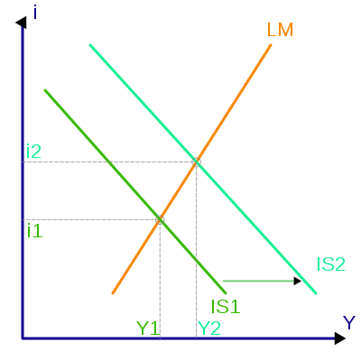
Factors that Shift the IS Schedule
I(r) + G = S(Y - T) + T

1. Government spending (incresase) will shift the schedule to the right.
The amount of the shift will be Change in G over the MPS (1-b).
2. An increase in Tax revenues will shift the IS schedule to the left by:
-b/(1-b)
3. An autonomous increase in investments will shift the IS Schedule to the right by:
1/(1-b) or 1/MPS
4. Open Economy: an autonomous increase in exports will shift the IS schedule to the right.

The IS Schedule: Summary

1. The IS curve slopes downward to the right.
2. The IS curve will be relatively flat if the interest elasticity of investment is relatively high (steep/low).
3. The IS curve will shift to the right when there is an increase in the level of government expenditures (left/decrease).
4. The IS curve will shift to the left when the level of taxes increases (right/declines).
5. An autonomous increase in investment expenditures will shift the IS curve to the right (decrease/left).
6. The IS curve will be relatively steeper the higher the MPS.

Quadrants:
Left and Above the LM schedule indicates an excess supply of money (interest rate too high for the money market equilibrium).
Right and above the IS schedule indicates an excess supply of output.

An Open Economy/BP Schedule
IS Equation for an open economy is stated as:
S(Y) + T + Z(Y) = I(r) + G + X
Thus Exports (X) is exogenous and Imports (Z) is a fraction of total income.
And thus in an open economy we need to notice that an increase in autonomous exports will shift the IS Schedule to the right. And an autonomous decline in import demand will shift the IS Schedule to the right assuming that there is an increase in domestic output consumption.

BP Schedule plots all interest rate-income combinations that result in balance of payments equilibrium at a given exchange rate. By balance of payments equilibrium is meant that the official reserves transaction balance is zero. Equation:
X(R) - Z(Y,R) + F(r) = 0
R is the exchange rate and F is the capital inflow.
Factors that shift the BP Schedule:

1. An increase in R (Exchange Rate-actually a depreciation of Currency- a worsening terms of trade) will shift the schedule horizontally to the right.
2. Exogenous increase in Exports or fall in Import demand will shift the BP Schedule to the right.

Points to the right (& below) indicate a deficit in the balance of payments.

Monetary and Fiscal Policy in an Open Economy: Fixed Exchange Rates
Monetary policy expansion under a Fixed Exchange rate will shift the LM curve to the Right and result in a BoP deficit (or any other action causing the LM to shift to right).

Fiscal expansionary policy will have an indeterminate effect on BoP depending on LM/BP slopes with regard to each other.
If the LM schedule is steeper it will result in a favorable BoP. And if the BP is steeper then BoP will be negative and the intersection will be to the right of the BP slope.

This follows since ceteris paribus the steeper the LM schedule, the larger the increase in interest rate (which produces the favorable capital inflow) and the smaller the increase in income (which produces the unfavorable effect on the trade balance) as a result of expansionary policy action.

Monetary and Fiscal Policy in an Open Economy: Flexible Exchange Rates
Monetary expansion will shift the LM curve to the right, but in a flexible exchange rate it also: exchange rates will rise and shift the BP schedule to the right and the higher exchange rate will shift the IS schedule to the right from exports rising and imports will fall.

With a flexible exchange rate, the rise in the exchange rate will futher stimulate income by increasing exports and reducing import demand (for a given income level). Monetary policy is therefore a more potent stabilization tool in a flexible exchange rate regime.

Again the effects of an increase in Fiscal Expansionary Policy is indeterminate:
When the LM curve is more steep than the BP curve (as in classical economics): then as Government spends more the IS shifts to the right. BoP is in a surplus rates must fall and thus shift the BP schedule to the left. The fall in exchange rate will also cause the IS schedule to shift leftward caused by lower level of exports and stimulate import demand. Thus if the LM curve is perfectly inelastic there would be no effect of expansionary policy.

On the other hand if BP schedule is steeper than the LM schedule then expansionary Fiscal Policy will result in BoP deficit causing exchange rates to rise and shift both the BP and the IS schedules to the right. And thus the multiplier effect is larger-although unlikely.

Note: a rise in exchange rates means an actual devaluation.